|
| Command: |
 Image Analysis > Quantification > PLS Regression > Designer Image Analysis > Quantification > PLS Regression > Designer |
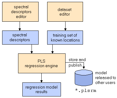
This tool allows the design of a PLS-based regression model. You first have to define and/or load a set of spectral descriptors and a set of training data. The training dataset specifies individual points in an image with known class quantitative values (e.g. concentrations). After the design-process the model can be stored and applied to other data sets.
| How To: |
- Load the spectral desciptors by clicking the
 button. button.
- Load the training set by clicking the
 button. If you have not yet created a set, do so by clicking the button. If you have not yet created a set, do so by clicking the  button in the main window and prepare your set, before you proceed. button in the main window and prepare your set, before you proceed.
- Set the number of factors to 20 or to the maximum of available descriptors.
- Click the "Calculate" button.
- Optimize the number of factors and verify your model by using the tabs in the lower part of the window.
- Store the optimum model for later application to unknown data.
|
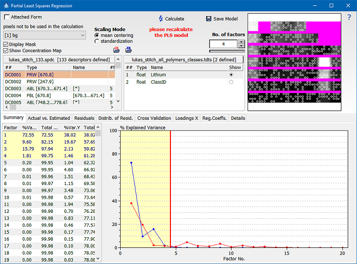
The upper part of the window shows the list of descriptors and a table containing the training data. The corresponding data points of the training dataset are depicted in the top right graph combined with the currently selected descpriptor as a background.
The following table gives an explanation to the tabs.
| Tab |
Description |
| Summary |
The table on the left hand side contains the explained variance for X and Y for each factor. Two additional columns show the integral over these values, starting from factor 1. The graph on the right hand side depicts the X values (blue) and Y values (red) over the corresponding factor number. The number of factors can be specified by either clicking on the graph or using the selection in the upper right window.
|
| Actual vs. Estimated |
The plot on the left hand side depicts the correlation between actual and estimated data. The plot on the right hand side depicts the concentration map for the currently selected quantitative value. Please note that the calculation of the concentration map can be time-consuming and can be deactivated by deselecting the check box "Show Concentraion Map".
|
| Residuals |
This graph depicts the residual value for each test data point.
|
| Distrib. of Resid. |
This graph depicts the histogram of the residuals.
|
| Cross Validation |
This tool allows a cross validation of the calculated model. The calculation can be initialized by clicking on the "Start Cross Validation" button and can be aborted by clicking the "Abort" button. "Test Set Size" signifies the number of data points, that shall be excluded from the original training set. The result of the cross validation is depicted in the graph window, where the different values of the root mean square error of prediction [RMS(EP)] are plotted for each factor number. The table on the left hand side summarizes these results as mean error and standard deviation.
|
| Loadings X |
This graph depicts the loadings of the spectral descriptors used to set up the model. By moving the mouse over the peaks, one can read the corresponding values from the boxes at the bottom left.
|
| Reg. Coeffs. |
This graph depicts the model coefficient for each spectral descriptor. By moving the mouse over the peaks, one can read the corresponding values from the boxes at the bottom left.
|
| Details. |
On this tab all the numeric details of the regression model are listed.
|
|
 Image Processing

